Latent Growth Curve Modelling (LT7)
Preliminaries
library(lme4)
library(lavaan)
library(interactions)
library(tidyverse)
library(sjmisc)
library(semPlot)
Introduction
Latent growth curve (LGC) models are in a sense, just a different form of the longitudinal multilevel model we looked at before reading week. In some ways they are more flexible, mostly because they are conducted in the structural equation modeling framework that allows for indirect, and other more complicated process models. Mainly, though, their main application is to developmental research where people are measured over a considerable amount of time and their trajectories of change are the dependent variables of interest.
LGC models are a very popular SEM technique in the psychological and behavioral sciences, so it makes sense to become familiar with them. To best understand a growth curve model, I still think it’s instructive to see it from the multilevel model framework, where things are mostly interpretable from what you know about random intercepts and slope trajectories. We will do that here. First looking at addressing LT5’s research question using multilevel modelling and then doing the same analysis with LGC modeling.
Random effects
As a reminded of why we need this type of analysis: often data is clustered (e.g. students within schools or observations for individuals over time). The general linear model assumes independent observations, and in these situations we definitely do not have that. This is massive problem for estimates, as we saw in LT5.
One very popular way to deal with clustering are a class of models called multilevel models. They are some times called mixed models because there is a mixture of fixed effects and random effects. The fixed effects are the regression coefficients one has in standard modeling approaches. We saw how these work and are applied in LT5.
The random effects are especially important because they allow each cluster to have its own unique intercept and slope in addition to the overall fixed intercept and slope. The random effect fro any cluster is simply the cluster’s intercept and slope deviation from the overall intercept and slopes.
Fixed and Random Effects in Longitudinal Multilevel Modelling
As we’ve seen with our work on structural equation modeling, the latent variables capture common variance in a set of correlated items, usually with a mean, and some standard deviation. Well this is also what random effects are in mixed models (i.e., variance in a set of correlated intercepts or slopes), and it’s through this that we can start to get a sense of random effects as latent variables.
Fixed and Random Effects in MLM
We saw in the multilevel modeling framework that the multilevel equation for this set of effects can be expressed as:
Yti = Ma + (MB + WBi)*time + Wai + eti
Where Ma is the fixed intercept, MB is the fixed slope, WB is the random slope variance, Wa is the random intercept variance, and Y is the outcome variable for individual i at time point t. e is simply the error left over once the multilevel model is subtracted out (i.e., the error in simple ANOVA).
Fixed and Random Effects in Structural Equation Modelling
Rather than express this model in notation form, we can also express it in latent variable form, as we might do in SEM. Lets have a look at that:
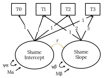
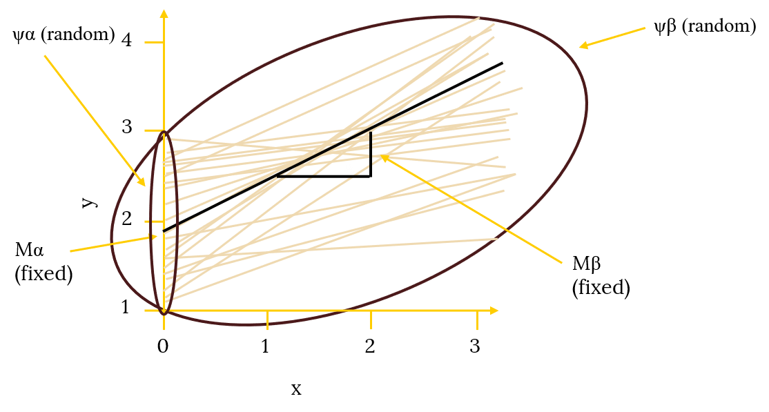
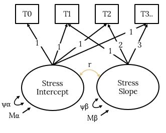
Fixed and Random Effects in LGCM
To all intents and purposes, this model is exactly the same as the multilevel model we have just expressed in notional format above. Just this time, the intercepts and slopes are represented by latent variables. We have a latent variable representing the random intercepts and a latent variable representing the random slopes. All loadings for the intercept latent variable are fixed at 1 so that the intercept latent variable has a mean that is the mean of the first time point (Ma). This is the fixed effect for the intercept. The intercept latent variable also has a variance that is the variability around the mean of the first time point (Wa). This is the random effect for the intercept.
The loadings for the slope latent variable are arbitrary, but should accurately reflect the time spacing, and typically, just like in the multilevel model, it is good to start at zero, so that the zero (the intercept) is the mean of the first time point. Hence, there is no loading for T0 because the T0 loading would be zero. Every loading for each time point thereafter is 1, 2, 3 and so on for a linear trajectory (we could take the square of these time points for a quadratic trend, for example, but we will stick with linear trajectories for now). In this way, the slope factor is simply the regression of time on our outcome variable (in this example, shame). The slope latent variable mean being the mean slope or trajectory of time (MB). This the fixed effect of the slope. The slope latent variable variance being the variability in the trajectories (WB).
The cool thing about modeling longitudinal trajectories in this way is that we can add latent variable predictors to explain latent variable variance in the intercept or slopes. In this way, we are modeling relationships in the absence of error and we know that is crucially important for regression.
Okay lets run this LGC with the same data we looked at in LT5.
Longitudinal Data: Time Points Nested Within People
Recall from LT5 that the data we worked with for the analysis of longitudinal data is the stress data from Ram et al (2012). This is a classic diary design, whereby the researchers were interested to know the effects of personalty of daily levels of stress. The citation for the work is here:
Ram, N., Conroy, D. E., Pincus, A. L., Hyde, A. L., & Molloy, L. E. (2012). Tethering theory to method: Using measures of intraindividual variability to operationalize individuals’ dynamic characteristics. In G. Hancock & J. Harring (Eds.), Advances in longitudinal methods in the social and behavioral sciences (pp. 81-110). New York: Information Age.
As we saw in LT5, longitudinal data is a special case of nested data where time points are nested within people. In this case, the data Ram collected was from a diary study of workers in a big tech firm. Once a day for eight days, researchers measured employees’ levels of stress and negative affect (this is why it is called a diary study, participants typically complete a daily diary).
At the end of the study, they took one measure of neuroticism. In this way, the researchers have data at two-levels. At level two, they had between person differences in neuroticism (i.e., how people differ from the sample mean in terms of their neuroticism). At level one, they had within-person differences in stress and negative affect (i.e., how people differ from their own mean stress and negative affect on a particular day).

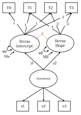
A Two-Level Nested Longitudinal Data-Structure
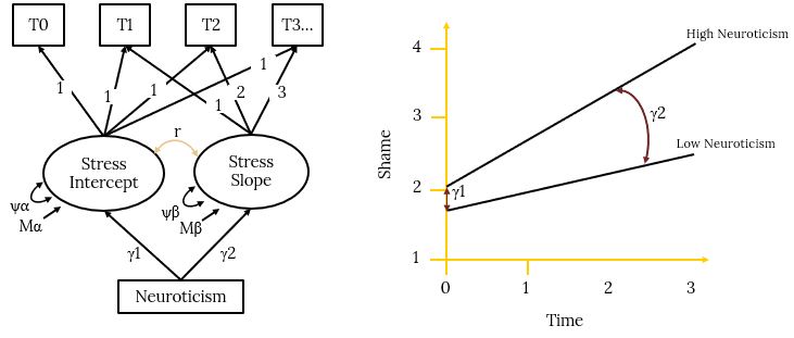
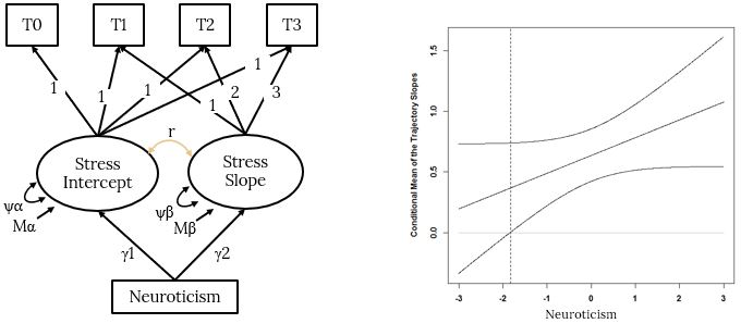
The researchers were interested to know whether neuroticism in the workplace predicted the change trajectories of stress over the period of study
To address this question with LGC we need to create our growth curve model of stress and then see whether neuroticism explains variance in the slope trajectories.
A LGCM of Stress with Neuroticism Predicting the Stress Intercepts and Slopes
The Data
As always, let’s first load in the data here:
stress <- read_csv("C:/Users/CURRANT/Dropbox/Work/LSE/PB230/LT7/Workshop/stress.csv")##
## -- Column specification -----------------------------------------------------------------------------------------------------------------------
## cols(
## id = col_double(),
## day = col_double(),
## negaff = col_double(),
## stress = col_double(),
## neurotic = col_double(),
## stress_personmean = col_double(),
## negaff_personmean = col_double(),
## neurotic_gmc = col_double(),
## stress_gmc = col_double(),
## stress_pmc = col_double(),
## negaff_pmc = col_double()
## )head(stress, 16)## # A tibble: 16 x 11
## id day negaff stress neurotic stress_personme~ negaff_personme~
## <dbl> <dbl> <dbl> <dbl> <dbl> <dbl> <dbl>
## 1 101 0 3 1.5 2 1.06 1.5
## 2 101 1 2.3 1.25 2 1.06 1.5
## 3 101 2 1 0.5 2 1.06 1.5
## 4 101 3 1.3 1 2 1.06 1.5
## 5 101 4 1.1 1.25 2 1.06 1.5
## 6 101 5 1 1.25 2 1.06 1.5
## 7 101 6 1.2 0.5 2 1.06 1.5
## 8 101 7 1.1 1.25 2 1.06 1.5
## 9 102 0 1.4 0.5 2 0.781 2.22
## 10 102 1 1.6 0 2 0.781 2.22
## 11 102 2 2.6 0 2 0.781 2.22
## 12 102 3 2.8 2.25 2 0.781 2.22
## 13 102 4 1.7 0 2 0.781 2.22
## 14 102 5 2.65 0.25 2 0.781 2.22
## 15 102 6 2.2 1.25 2 0.781 2.22
## 16 102 7 2.8 2 2 0.781 2.22
## # ... with 4 more variables: neurotic_gmc <dbl>, stress_gmc <dbl>,
## # stress_pmc <dbl>, negaff_pmc <dbl>Estimating the Model Using MLM
Let’s estimate this as a multilevel model first using the lme4 package like last week. See if you can match the parameters from our simulated data to the output.
First just the stress trajectory model with the first time point centered day variable. This is equivalent to the growth curve model. Essentially what we are doing here is examining the mean (fixed) trajectory of stress across the study, and the person-to-person variability (random) around that fixed effect. Is stress changing and do different people change in different ways?
time.stress.fit <- lmer(formula = stress ~ 1 + day + (1 + day|id), REML=FALSE, data=stress)## Warning in checkConv(attr(opt, "derivs"), opt$par, ctrl = control$checkConv, :
## Model failed to converge with max|grad| = 0.00345471 (tol = 0.002, component 1)summary(time.stress.fit)## Linear mixed model fit by maximum likelihood ['lmerMod']
## Formula: stress ~ 1 + day + (1 + day | id)
## Data: stress
##
## AIC BIC logLik deviance df.resid
## 2602.4 2634.1 -1295.2 2590.4 1439
##
## Scaled residuals:
## Min 1Q Median 3Q Max
## -3.1112 -0.6479 -0.0737 0.5605 3.9987
##
## Random effects:
## Groups Name Variance Std.Dev. Corr
## id (Intercept) 0.174765 0.41805
## day 0.002812 0.05303 -0.14
## Residual 0.264434 0.51423
## Number of obs: 1445, groups: id, 190
##
## Fixed effects:
## Estimate Std. Error t value
## (Intercept) 1.386688 0.039095 35.470
## day 0.001260 0.007091 0.178
##
## Correlation of Fixed Effects:
## (Intr)
## day -0.493
## optimizer (nloptwrap) convergence code: 0 (OK)
## Model failed to converge with max|grad| = 0.00345471 (tol = 0.002, component 1)confint(time.stress.fit, method="boot", nsim=100)## Computing bootstrap confidence intervals ...##
## 2 warning(s): Model failed to converge with max|grad| = 0.00201849 (tol = 0.002, component 1) (and others)## 2.5 % 97.5 %
## .sig01 0.31796927 0.48158117
## .sig02 -0.43218069 0.79935000
## .sig03 0.01255386 0.06961895
## .sigma 0.49331758 0.53313646
## (Intercept) 1.29464105 1.48863515
## day -0.01582625 0.01525968We saw that the slopes for stress were essentially flat according to the fixed effect (MB = .001), but there was significant person-to-person variability around that mean trajectory (WB = .05, 95% Ci = .02, .07). This was our justification for throwing neuroticism in the model as a between-person predictor of this variance.
Let’s run that model now with neuroticism interacting with day to predict the random slopes of stress:
time.stress.fit2 <- lmer(formula = stress ~ 1 + day + neurotic_gmc + day*neurotic_gmc + (1 + day|id), data=stress)
summary(time.stress.fit2)
## Linear mixed model fit by REML ['lmerMod']
## Formula: stress ~ 1 + day + neurotic_gmc + day * neurotic_gmc + (1 + day |
## id)
## Data: stress
##
## REML criterion at convergence: 2599.3
##
## Scaled residuals:
## Min 1Q Median 3Q Max
## -3.1029 -0.6566 -0.0703 0.5673 4.0427
##
## Random effects:
## Groups Name Variance Std.Dev. Corr
## id (Intercept) 0.152930 0.39106
## day 0.002681 0.05178 -0.05
## Residual 0.264449 0.51425
## Number of obs: 1445, groups: id, 190
##
## Fixed effects:
## Estimate Std. Error t value
## (Intercept) 1.386468 0.037591 36.883
## day 0.001229 0.007044 0.175
## neurotic_gmc -0.165306 0.039405 -4.195
## day:neurotic_gmc 0.015582 0.007372 2.114
##
## Correlation of Fixed Effects:
## (Intr) day nrtc_g
## day -0.474
## neurotc_gmc 0.000 0.002
## dy:nrtc_gmc 0.002 -0.019 -0.474confint(time.stress.fit2, method="boot", nsim=100)## Computing bootstrap confidence intervals ...##
## 2 warning(s): Model failed to converge with max|grad| = 0.00207401 (tol = 0.002, component 1) (and others)## 2.5 % 97.5 %
## .sig01 0.290024250 0.45649065
## .sig02 -0.316280694 0.79129753
## .sig03 0.025796869 0.06691275
## .sigma 0.497658084 0.53678546
## (Intercept) 1.304845265 1.46870861
## day -0.017874828 0.01728617
## neurotic_gmc -0.251587174 -0.07857423
## day:neurotic_gmc 0.004049417 0.02993046Of interest her was the interaction of neuroticism with day. We can see that the estimate for this interaction was .02 with a 95% confidence interval that does not include zero (.0002, .03). We then plotted this interaction:
johnson_neyman(model=time.stress.fit2, pred=day, modx=neurotic_gmc)## JOHNSON-NEYMAN INTERVAL
##
## When neurotic_gmc is OUTSIDE the interval [-3.15, 1.79], the slope of day
## is p < .05.
##
## Note: The range of observed values of neurotic_gmc is [-2.02, 1.98]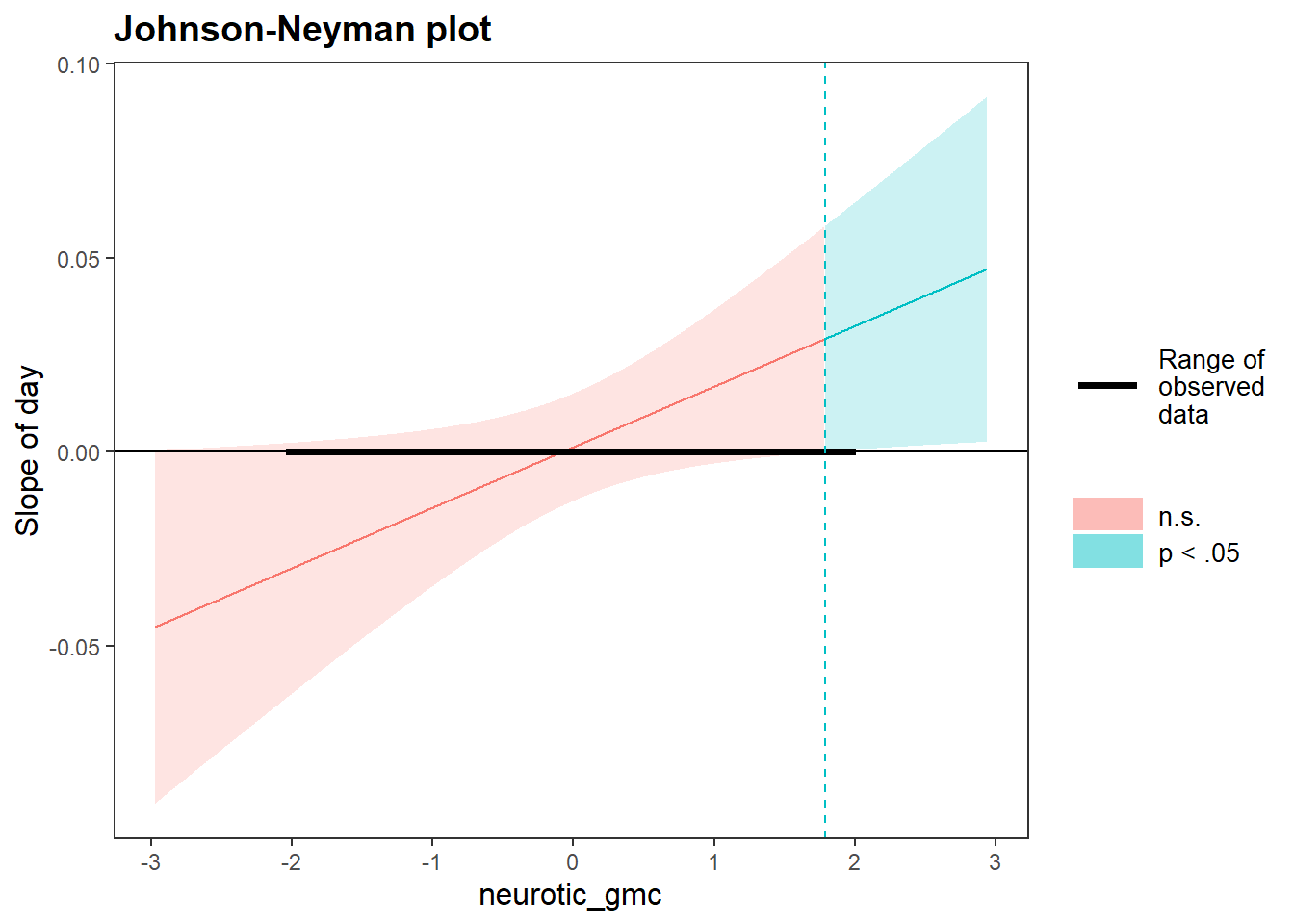
To show that the trajectories of stress were positive (i.e., stress increased over time) among people with higher levels of neuroticism.
Let’s now do this analysis using latent growth curve modeling.
Doing Latent Growth Curve Analysis
As we have been doing for latent variable analysis, we’ll use lavaan to conduct LGC modeling, but now the code will look a bit strange compared to what we’re used to because we have to fix the factor loadings to specific values in order to make it work.
This also leads to non-standard output relative to other SEM models, as there is nothing to estimate for the many fixed parameters.
Specifically, we’ll have a latent variable representing the random intercepts, as well as one representing the random slopes. All loadings for the intercept factor are 1. The loadings for the effect of time run from 0 to 7, just like in the multilevel model.
Data Structure
As can probably be guessed, our data needs to be in wide format to contain the time points as measured variables. Here, each row represents a person and we have separate columns for each time point of the target variable, as opposed to the long format we used in the previous multilevel model. We can use the spread function from tidyr to help with that.
stress_wide <- stress %>%
  dplyr::select(id,day,stress,neurotic) %>%
  spread(day, stress) %>%
  rename_at(vars(-id), function(x) paste0('y', x))
head(stress_wide)
## # A tibble: 6 x 11
## id yneurotic y0 y1 y2 y3 y4 y5 y6 y7 `y<NA>`
## <dbl> <dbl> <dbl> <dbl> <dbl> <dbl> <dbl> <dbl> <dbl> <dbl> <dbl>
## 1 101 2 1.5 1.25 0.5 1 1.25 1.25 0.5 1.25 NA
## 2 102 2 0.5 0 0 2.25 0 0.25 1.25 2 NA
## 3 103 2.5 1.25 NA NA 1 1.25 0.75 2 1.25 NA
## 4 104 2.5 1.5 2.25 1.75 1.5 2.25 1.75 1.75 1.75 NA
## 5 105 3.5 1.5 1.5 1 1.25 2.75 2.5 1.75 1.75 NA
## 6 106 1.5 0.75 0.75 2.25 1.75 0 1.5 2 0 NABuilding the LGC Model for Stress
Now we’re ready to run the LGC model. This is essentially the same model as the first multilevel model tested above. It asks: Is stress changing and do different people change in different ways? Only this time, we are capturing the fixed and random effects with latent variables.
LGCM of Stress
When building the model, we will use the typical “=~” command to stipulate our latent variables. To give our time points their specific factor loadings, we will use "*". But otherwise, we are just building a latent variable model, just like we have been doing in the SEM content. Lets build that model now, specifying the unique factor loadings we want for each time point on each of the intercept and slope latent variables:
lgc.model <- "
    # intercept and slope with fixed coefficients
    intercept =~ 1*y0 + 1*y1 + 1*y2 + 1*y3 + 1*y4 + 1*y5 + 1*y6 + 1*y7
    slope =~ 0*y0 + 1*y1 + 2*y2 + 3*y3 + 4*y4 + 5*y5 + 6*y6 + 7*y7
"
Fitting the LGCM
Note that lavaan has a specific function, growth, to use for these models. It doesn’t spare us any effort for the model coding (as above), but does make it unnecessary to set various things with the sem function:
lgc.fit <- growth(lgc.model, data=stress_wide)
summary(lgc.fit, fit.measures=TRUE, standardized=TRUE)
## lavaan 0.6-7 ended normally after 37 iterations
##
## Estimator ML
## Optimization method NLMINB
## Number of free parameters 13
##
## Used Total
## Number of observations 159 191
##
## Model Test User Model:
##
## Test statistic 59.157
## Degrees of freedom 31
## P-value (Chi-square) 0.002
##
## Model Test Baseline Model:
##
## Test statistic 454.707
## Degrees of freedom 28
## P-value 0.000
##
## User Model versus Baseline Model:
##
## Comparative Fit Index (CFI) 0.934
## Tucker-Lewis Index (TLI) 0.940
##
## Loglikelihood and Information Criteria:
##
## Loglikelihood user model (H0) -1125.019
## Loglikelihood unrestricted model (H1) -1095.441
##
## Akaike (AIC) 2276.039
## Bayesian (BIC) 2315.935
## Sample-size adjusted Bayesian (BIC) 2274.782
##
## Root Mean Square Error of Approximation:
##
## RMSEA 0.076
## 90 Percent confidence interval - lower 0.046
## 90 Percent confidence interval - upper 0.105
## P-value RMSEA <= 0.05 0.076
##
## Standardized Root Mean Square Residual:
##
## SRMR 0.078
##
## Parameter Estimates:
##
## Standard errors Standard
## Information Expected
## Information saturated (h1) model Structured
##
## Latent Variables:
## Estimate Std.Err z-value P(>|z|) Std.lv Std.all
## intercept =~
## y0 1.000 0.435 0.646
## y1 1.000 0.435 0.640
## y2 1.000 0.435 0.688
## y3 1.000 0.435 0.633
## y4 1.000 0.435 0.630
## y5 1.000 0.435 0.626
## y6 1.000 0.435 0.621
## y7 1.000 0.435 0.590
## slope =~
## y0 0.000 0.000 0.000
## y1 1.000 0.056 0.082
## y2 2.000 0.111 0.176
## y3 3.000 0.167 0.243
## y4 4.000 0.223 0.323
## y5 5.000 0.279 0.401
## y6 6.000 0.334 0.478
## y7 7.000 0.390 0.529
##
## Covariances:
## Estimate Std.Err z-value P(>|z|) Std.lv Std.all
## intercept ~~
## slope -0.004 0.005 -0.804 0.421 -0.161 -0.161
##
## Intercepts:
## Estimate Std.Err z-value P(>|z|) Std.lv Std.all
## .y0 0.000 0.000 0.000
## .y1 0.000 0.000 0.000
## .y2 0.000 0.000 0.000
## .y3 0.000 0.000 0.000
## .y4 0.000 0.000 0.000
## .y5 0.000 0.000 0.000
## .y6 0.000 0.000 0.000
## .y7 0.000 0.000 0.000
## intercept 1.360 0.043 31.507 0.000 3.130 3.130
## slope 0.004 0.008 0.508 0.612 0.069 0.069
##
## Variances:
## Estimate Std.Err z-value P(>|z|) Std.lv Std.all
## .y0 0.264 0.038 7.023 0.000 0.264 0.583
## .y1 0.277 0.036 7.659 0.000 0.277 0.601
## .y2 0.213 0.028 7.634 0.000 0.213 0.535
## .y3 0.278 0.035 8.038 0.000 0.278 0.590
## .y4 0.269 0.034 7.967 0.000 0.269 0.565
## .y5 0.255 0.033 7.728 0.000 0.255 0.529
## .y6 0.236 0.033 7.232 0.000 0.236 0.482
## .y7 0.256 0.038 6.754 0.000 0.256 0.473
## intercept 0.189 0.034 5.534 0.000 1.000 1.000
## slope 0.003 0.001 2.798 0.005 1.000 1.000Most of the output is blank, which is needless clutter, but we do get the same five parameter values we are interested in.
Start with the ‘intercepts’:
It might be odd to call your fixed effects ‘intercepts’, but that is where lavaan prints the fixed effects for our intercepts and slopes. This makes sense if we are thinking of it as a multilevel model as depicted previously, where we actually broke out the random effects as a separate model. The estimates here for the fixed intercept (1.360) and fixed slope (.004) are more or less the same as our multilevel model model estimates (the trivial differences are due to different estimation approaches). We can also see that, just like our multilevel model, the mean (fixed) slope is not different from zero (i.e., p > .05) indicating that the average trajectory for stress is pretty much flat.
Now let’s look at the variance estimates:
The estimation of residual variance for each time point in the LGC is the variance in the differences between observed time point stress scores and the model predicted stress score for that measurement occasion. We could fix them to be identical here, or conversely allow them to be estimated in the multilevel model framework (multilevel models by default assume the same variance for each time point). Thats another reasons why the results are not identical, by the way.
The main thing to worry about here, though, is the variance of the intercepts and slopes. There are the random effects for the model. Just like in the multilevel model, we can see that the variance of the intercepts (.189) and, importantly, the slopes (.003) are greater than zero (i.e., p > .05). So even though the average stress trajectory is flat, there is significant variability around that average.
The covariance is the relationship between the random intercept and random slope, just like in the multilevel model.
We also have model fit indexes that are interpreted in exactly the same way we have been doing to date for SEM. We have CFI = .93, TLI .94, RMSEA = .08, and SRMR = .08. Thats pretty good! If there was some missfit here, it might be that we need to remove the intercept or slope factor (if no variance) or perhaps model the trajectories using quadratic or cubic terms. None of these are needed here though.
Given we have substantial variance in the random intercepts and slopes within out LGC model, we should add neuroticism to ascertain whether i can explain this variance.
Adding a Categorical Predictor to the LGC Model
In explaining intercept and slope variance in a LGC model, we can add either categorical or continuous predictors. And these predictors can be observed or latent variables. This flexibility is what gives LGC modeling its advantage over multilevel modeling.
Lets begin with a categorical predictor. Adding a categorical variable would allow for different trajectories of stress across different groups of neuroticism. To begin with, lets create a categorical neuroticism variable, which does a simple media split such that people with neuroticism scores above the median (i.e., > 3) are coded 1, and those below the median (i.e., < 3) are coded 0.
stress_wide <- dicho(stress_wide, yneurotic, dich.by = 3) We now have a new variable, yneurotic_d which contains high and low scores on the neuroticism scale. When we regress this variable on our latent intercept and slope variables from the stress LGC model, we split the variance in stress intercepts and slopes by high and low neuroticism:
LGCM of Stress with Categorical Predictor
All we do to add this predictor to the model is regress it on the intercept and slope latent variables using ~. Simple!
lgc.cat.model <- "
    # intercept and slope with fixed coefficients
    intercept =~ 1*y0 + 1*y1 + 1*y2 + 1*y3 + 1*y4 + 1*y5 + 1*y6 + 1*y7
    slope =~ 0*y0 + 1*y1 + 2*y2 + 3*y3 + 4*y4 + 5*y5 + 6*y6 + 7*y7
    # regress categorcial predictor on the slopes and intercepts
    intercept ~ yneurotic_d
    slope ~ yneurotic_d
"
Then we simply fit that model and inspect the estimates remembering this time to request the confidence intervals from bootstrap given the structural relationship now in the model:
lgc.cat.fit <- growth(lgc.cat.model, data=stress_wide, se = "bootstrap", bootstrap = 100)
summary(lgc.cat.fit, fit.measures=TRUE, standardized=TRUE)
## lavaan 0.6-7 ended normally after 54 iterations
##
## Estimator ML
## Optimization method NLMINB
## Number of free parameters 15
##
## Used Total
## Number of observations 159 191
##
## Model Test User Model:
##
## Test statistic 67.030
## Degrees of freedom 37
## P-value (Chi-square) 0.002
##
## Model Test Baseline Model:
##
## Test statistic 471.859
## Degrees of freedom 36
## P-value 0.000
##
## User Model versus Baseline Model:
##
## Comparative Fit Index (CFI) 0.931
## Tucker-Lewis Index (TLI) 0.933
##
## Loglikelihood and Information Criteria:
##
## Loglikelihood user model (H0) -1120.380
## Loglikelihood unrestricted model (H1) -1086.865
##
## Akaike (AIC) 2270.759
## Bayesian (BIC) 2316.793
## Sample-size adjusted Bayesian (BIC) 2269.310
##
## Root Mean Square Error of Approximation:
##
## RMSEA 0.071
## 90 Percent confidence interval - lower 0.043
## 90 Percent confidence interval - upper 0.098
## P-value RMSEA <= 0.05 0.098
##
## Standardized Root Mean Square Residual:
##
## SRMR 0.073
##
## Parameter Estimates:
##
## Standard errors Bootstrap
## Number of requested bootstrap draws 100
## Number of successful bootstrap draws 100
##
## Latent Variables:
## Estimate Std.Err z-value P(>|z|) Std.lv Std.all
## intercept =~
## y0 1.000 0.435 0.650
## y1 1.000 0.435 0.642
## y2 1.000 0.435 0.688
## y3 1.000 0.435 0.631
## y4 1.000 0.435 0.630
## y5 1.000 0.435 0.626
## y6 1.000 0.435 0.622
## y7 1.000 0.435 0.589
## slope =~
## y0 0.000 0.000 0.000
## y1 1.000 0.056 0.083
## y2 2.000 0.112 0.177
## y3 3.000 0.168 0.244
## y4 4.000 0.224 0.325
## y5 5.000 0.280 0.403
## y6 6.000 0.336 0.481
## y7 7.000 0.392 0.531
##
## Regressions:
## Estimate Std.Err z-value P(>|z|) Std.lv Std.all
## intercept ~
## yneurotic_d 0.262 0.083 3.143 0.002 0.603 0.298
## slope ~
## yneurotic_d -0.025 0.014 -1.790 0.073 -0.438 -0.216
##
## Covariances:
## Estimate Std.Err z-value P(>|z|) Std.lv Std.all
## .intercept ~~
## .slope -0.002 0.005 -0.505 0.613 -0.108 -0.108
##
## Intercepts:
## Estimate Std.Err z-value P(>|z|) Std.lv Std.all
## .y0 0.000 0.000 0.000
## .y1 0.000 0.000 0.000
## .y2 0.000 0.000 0.000
## .y3 0.000 0.000 0.000
## .y4 0.000 0.000 0.000
## .y5 0.000 0.000 0.000
## .y6 0.000 0.000 0.000
## .y7 0.000 0.000 0.000
## .intercept 0.987 0.127 7.751 0.000 2.270 2.270
## .slope 0.039 0.022 1.767 0.077 0.692 0.692
##
## Variances:
## Estimate Std.Err z-value P(>|z|) Std.lv Std.all
## .y0 0.259 0.037 7.082 0.000 0.259 0.578
## .y1 0.275 0.046 5.946 0.000 0.275 0.599
## .y2 0.214 0.022 9.592 0.000 0.214 0.535
## .y3 0.282 0.048 5.896 0.000 0.282 0.594
## .y4 0.269 0.039 6.918 0.000 0.269 0.565
## .y5 0.255 0.035 7.241 0.000 0.255 0.529
## .y6 0.235 0.035 6.637 0.000 0.235 0.481
## .y7 0.259 0.045 5.813 0.000 0.259 0.475
## .intercept 0.172 0.025 6.809 0.000 0.911 0.911
## .slope 0.003 0.001 2.079 0.038 0.953 0.953parameterestimates(lgc.cat.fit, boot.ci.type = "perc", standardized = TRUE)## lhs op rhs est se z pvalue ci.lower ci.upper
## 1 intercept =~ y0 1.000 0.000 NA NA 1.000 1.000
## 2 intercept =~ y1 1.000 0.000 NA NA 1.000 1.000
## 3 intercept =~ y2 1.000 0.000 NA NA 1.000 1.000
## 4 intercept =~ y3 1.000 0.000 NA NA 1.000 1.000
## 5 intercept =~ y4 1.000 0.000 NA NA 1.000 1.000
## 6 intercept =~ y5 1.000 0.000 NA NA 1.000 1.000
## 7 intercept =~ y6 1.000 0.000 NA NA 1.000 1.000
## 8 intercept =~ y7 1.000 0.000 NA NA 1.000 1.000
## 9 slope =~ y0 0.000 0.000 NA NA 0.000 0.000
## 10 slope =~ y1 1.000 0.000 NA NA 1.000 1.000
## 11 slope =~ y2 2.000 0.000 NA NA 2.000 2.000
## 12 slope =~ y3 3.000 0.000 NA NA 3.000 3.000
## 13 slope =~ y4 4.000 0.000 NA NA 4.000 4.000
## 14 slope =~ y5 5.000 0.000 NA NA 5.000 5.000
## 15 slope =~ y6 6.000 0.000 NA NA 6.000 6.000
## 16 slope =~ y7 7.000 0.000 NA NA 7.000 7.000
## 17 intercept ~ yneurotic_d 0.262 0.083 3.143 0.002 0.073 0.405
## 18 slope ~ yneurotic_d -0.025 0.014 -1.790 0.073 -0.047 0.008
## 19 y0 ~~ y0 0.259 0.037 7.082 0.000 0.189 0.346
## 20 y1 ~~ y1 0.275 0.046 5.946 0.000 0.191 0.384
## 21 y2 ~~ y2 0.214 0.022 9.592 0.000 0.166 0.252
## 22 y3 ~~ y3 0.282 0.048 5.896 0.000 0.196 0.393
## 23 y4 ~~ y4 0.269 0.039 6.918 0.000 0.191 0.343
## 24 y5 ~~ y5 0.255 0.035 7.241 0.000 0.189 0.337
## 25 y6 ~~ y6 0.235 0.035 6.637 0.000 0.167 0.305
## 26 y7 ~~ y7 0.259 0.045 5.813 0.000 0.177 0.353
## 27 intercept ~~ intercept 0.172 0.025 6.809 0.000 0.116 0.216
## 28 slope ~~ slope 0.003 0.001 2.079 0.038 0.000 0.006
## 29 intercept ~~ slope -0.002 0.005 -0.505 0.613 -0.011 0.007
## 30 yneurotic_d ~~ yneurotic_d 0.244 0.000 NA NA 0.244 0.244
## 31 y0 ~1 0.000 0.000 NA NA 0.000 0.000
## 32 y1 ~1 0.000 0.000 NA NA 0.000 0.000
## 33 y2 ~1 0.000 0.000 NA NA 0.000 0.000
## 34 y3 ~1 0.000 0.000 NA NA 0.000 0.000
## 35 y4 ~1 0.000 0.000 NA NA 0.000 0.000
## 36 y5 ~1 0.000 0.000 NA NA 0.000 0.000
## 37 y6 ~1 0.000 0.000 NA NA 0.000 0.000
## 38 y7 ~1 0.000 0.000 NA NA 0.000 0.000
## 39 yneurotic_d ~1 1.421 0.000 NA NA 1.421 1.421
## 40 intercept ~1 0.987 0.127 7.751 0.000 0.780 1.291
## 41 slope ~1 0.039 0.022 1.767 0.077 -0.007 0.077
## std.lv std.all std.nox
## 1 0.435 0.650 0.650
## 2 0.435 0.642 0.642
## 3 0.435 0.688 0.688
## 4 0.435 0.631 0.631
## 5 0.435 0.630 0.630
## 6 0.435 0.626 0.626
## 7 0.435 0.622 0.622
## 8 0.435 0.589 0.589
## 9 0.000 0.000 0.000
## 10 0.056 0.083 0.083
## 11 0.112 0.177 0.177
## 12 0.168 0.244 0.244
## 13 0.224 0.325 0.325
## 14 0.280 0.403 0.403
## 15 0.336 0.481 0.481
## 16 0.392 0.531 0.531
## 17 0.603 0.298 0.603
## 18 -0.438 -0.216 -0.438
## 19 0.259 0.578 0.578
## 20 0.275 0.599 0.599
## 21 0.214 0.535 0.535
## 22 0.282 0.594 0.594
## 23 0.269 0.565 0.565
## 24 0.255 0.529 0.529
## 25 0.235 0.481 0.481
## 26 0.259 0.475 0.475
## 27 0.911 0.911 0.911
## 28 0.953 0.953 0.953
## 29 -0.108 -0.108 -0.108
## 30 0.244 1.000 0.244
## 31 0.000 0.000 0.000
## 32 0.000 0.000 0.000
## 33 0.000 0.000 0.000
## 34 0.000 0.000 0.000
## 35 0.000 0.000 0.000
## 36 0.000 0.000 0.000
## 37 0.000 0.000 0.000
## 38 0.000 0.000 0.000
## 39 1.421 2.879 1.421
## 40 2.270 2.270 2.270
## 41 0.692 0.692 0.692First of all, the model fit looks pretty good. We have CFI = .93, TLI .93, RMSEA = .07, and SRMR = .07. Of interest here are the regressions, first of the latent stress intercept on categorical neuroticism and second of the latent stress slope on categorical neuroticism.
We can see that the regression of stress intercepts on neuroticism is .26 and this is a significant effect according the the 95% bootstrap confidence interval (95% Ci = .11, .41). The interpretation of this regression is that people with high neuroticism start the study (i.e., time point 0) with stress levels that are .26 units higher than people with low neuroticism. Interesting, but what we really want to know is whether the trajectories of stress differ across neuroticism groups.
To answer that question we need to look to the regression of stress slopes on neuroticism. Here we have an estimate of -.03 and this is not a significant effect according the the 95% bootstrap confidence interval (95% Ci = -.05, .01). The interpretation of this regression is that people with high neuroticism have stress trajectories that are -.03 units smaller (shallower, less steep) than people with low neuroticism.
Adding a Continuous Predictor to the LGC Model
If you cast your mind back to last year when we split off continuous variables, we saw that doing so was a pretty bad idea because we are shrinking the variance in our x variable and thereby reducing the amount of error we could potentially explain in y. For this reason, it is always better to use the full range of a continuous variable. So lets now look to see if our continuous neuroticism variable can explain variability in the latent stress intercept and slope variables from the LGC model. In thsi way, we can ascertain whether the trajectory slopes of stress difference across the full range of neuroticism.
LGCM of Stress with Continuous Predictor
For this model we simply swap out yneurotic_d from the last model and replace it with yneurotic. Let’s build that model now:
lgc.con.model <- "
    # intercept and slope with fixed coefficients
    intercept =~ 1*y0 + 1*y1 + 1*y2 + 1*y3 + 1*y4 + 1*y5 + 1*y6 + 1*y7
    slope =~ 0*y0 + 1*y1 + 2*y2 + 3*y3 + 4*y4 + 5*y5 + 6*y6 + 7*y7
    # regress continuous predictor on the slopes and intercepts
    intercept ~ yneurotic
    slope ~ yneurotic
"
Now lets fit that model in exactly the same way we did for the categorical predictor:
lgc.con.fit <- growth(lgc.con.model, data=stress_wide, se = "bootstrap", bootstrap = 100)
summary(lgc.con.fit, fit.measures=TRUE, standardized=TRUE)
## lavaan 0.6-7 ended normally after 55 iterations
##
## Estimator ML
## Optimization method NLMINB
## Number of free parameters 15
##
## Used Total
## Number of observations 159 191
##
## Model Test User Model:
##
## Test statistic 67.975
## Degrees of freedom 37
## P-value (Chi-square) 0.001
##
## Model Test Baseline Model:
##
## Test statistic 477.339
## Degrees of freedom 36
## P-value 0.000
##
## User Model versus Baseline Model:
##
## Comparative Fit Index (CFI) 0.930
## Tucker-Lewis Index (TLI) 0.932
##
## Loglikelihood and Information Criteria:
##
## Loglikelihood user model (H0) -1118.112
## Loglikelihood unrestricted model (H1) -1084.125
##
## Akaike (AIC) 2266.225
## Bayesian (BIC) 2312.258
## Sample-size adjusted Bayesian (BIC) 2264.775
##
## Root Mean Square Error of Approximation:
##
## RMSEA 0.073
## 90 Percent confidence interval - lower 0.045
## 90 Percent confidence interval - upper 0.099
## P-value RMSEA <= 0.05 0.087
##
## Standardized Root Mean Square Residual:
##
## SRMR 0.073
##
## Parameter Estimates:
##
## Standard errors Bootstrap
## Number of requested bootstrap draws 100
## Number of successful bootstrap draws 100
##
## Latent Variables:
## Estimate Std.Err z-value P(>|z|) Std.lv Std.all
## intercept =~
## y0 1.000 0.435 0.655
## y1 1.000 0.435 0.642
## y2 1.000 0.435 0.687
## y3 1.000 0.435 0.630
## y4 1.000 0.435 0.631
## y5 1.000 0.435 0.626
## y6 1.000 0.435 0.622
## y7 1.000 0.435 0.588
## slope =~
## y0 0.000 0.000 0.000
## y1 1.000 0.056 0.083
## y2 2.000 0.113 0.178
## y3 3.000 0.169 0.245
## y4 4.000 0.225 0.327
## y5 5.000 0.282 0.406
## y6 6.000 0.338 0.483
## y7 7.000 0.394 0.533
##
## Regressions:
## Estimate Std.Err z-value P(>|z|) Std.lv Std.all
## intercept ~
## yneurotic 0.163 0.042 3.891 0.000 0.374 0.358
## slope ~
## yneurotic -0.018 0.007 -2.588 0.010 -0.314 -0.300
##
## Covariances:
## Estimate Std.Err z-value P(>|z|) Std.lv Std.all
## .intercept ~~
## .slope -0.001 0.006 -0.264 0.792 -0.069 -0.069
##
## Intercepts:
## Estimate Std.Err z-value P(>|z|) Std.lv Std.all
## .y0 0.000 0.000 0.000
## .y1 0.000 0.000 0.000
## .y2 0.000 0.000 0.000
## .y3 0.000 0.000 0.000
## .y4 0.000 0.000 0.000
## .y5 0.000 0.000 0.000
## .y6 0.000 0.000 0.000
## .y7 0.000 0.000 0.000
## .intercept 0.877 0.128 6.833 0.000 2.017 2.017
## .slope 0.056 0.021 2.714 0.007 0.999 0.999
##
## Variances:
## Estimate Std.Err z-value P(>|z|) Std.lv Std.all
## .y0 0.252 0.035 7.132 0.000 0.252 0.571
## .y1 0.275 0.041 6.740 0.000 0.275 0.599
## .y2 0.216 0.022 9.696 0.000 0.216 0.538
## .y3 0.284 0.049 5.772 0.000 0.284 0.596
## .y4 0.269 0.040 6.726 0.000 0.269 0.565
## .y5 0.255 0.039 6.484 0.000 0.255 0.528
## .y6 0.235 0.031 7.499 0.000 0.235 0.481
## .y7 0.261 0.043 6.048 0.000 0.261 0.476
## .intercept 0.165 0.029 5.755 0.000 0.872 0.872
## .slope 0.003 0.002 1.912 0.056 0.910 0.910parameterestimates(lgc.con.fit, boot.ci.type = "perc", standardized = TRUE)## lhs op rhs est se z pvalue ci.lower ci.upper std.lv
## 1 intercept =~ y0 1.000 0.000 NA NA 1.000 1.000 0.435
## 2 intercept =~ y1 1.000 0.000 NA NA 1.000 1.000 0.435
## 3 intercept =~ y2 1.000 0.000 NA NA 1.000 1.000 0.435
## 4 intercept =~ y3 1.000 0.000 NA NA 1.000 1.000 0.435
## 5 intercept =~ y4 1.000 0.000 NA NA 1.000 1.000 0.435
## 6 intercept =~ y5 1.000 0.000 NA NA 1.000 1.000 0.435
## 7 intercept =~ y6 1.000 0.000 NA NA 1.000 1.000 0.435
## 8 intercept =~ y7 1.000 0.000 NA NA 1.000 1.000 0.435
## 9 slope =~ y0 0.000 0.000 NA NA 0.000 0.000 0.000
## 10 slope =~ y1 1.000 0.000 NA NA 1.000 1.000 0.056
## 11 slope =~ y2 2.000 0.000 NA NA 2.000 2.000 0.113
## 12 slope =~ y3 3.000 0.000 NA NA 3.000 3.000 0.169
## 13 slope =~ y4 4.000 0.000 NA NA 4.000 4.000 0.225
## 14 slope =~ y5 5.000 0.000 NA NA 5.000 5.000 0.282
## 15 slope =~ y6 6.000 0.000 NA NA 6.000 6.000 0.338
## 16 slope =~ y7 7.000 0.000 NA NA 7.000 7.000 0.394
## 17 intercept ~ yneurotic 0.163 0.042 3.891 0.000 0.071 0.249 0.374
## 18 slope ~ yneurotic -0.018 0.007 -2.588 0.010 -0.032 -0.006 -0.314
## 19 y0 ~~ y0 0.252 0.035 7.132 0.000 0.191 0.330 0.252
## 20 y1 ~~ y1 0.275 0.041 6.740 0.000 0.185 0.362 0.275
## 21 y2 ~~ y2 0.216 0.022 9.696 0.000 0.175 0.263 0.216
## 22 y3 ~~ y3 0.284 0.049 5.772 0.000 0.181 0.391 0.284
## 23 y4 ~~ y4 0.269 0.040 6.726 0.000 0.204 0.360 0.269
## 24 y5 ~~ y5 0.255 0.039 6.484 0.000 0.192 0.339 0.255
## 25 y6 ~~ y6 0.235 0.031 7.499 0.000 0.185 0.309 0.235
## 26 y7 ~~ y7 0.261 0.043 6.048 0.000 0.191 0.354 0.261
## 27 intercept ~~ intercept 0.165 0.029 5.755 0.000 0.113 0.222 0.872
## 28 slope ~~ slope 0.003 0.002 1.912 0.056 -0.001 0.006 0.910
## 29 intercept ~~ slope -0.001 0.006 -0.264 0.792 -0.013 0.011 -0.069
## 30 yneurotic ~~ yneurotic 0.915 0.000 NA NA 0.915 0.915 0.915
## 31 y0 ~1 0.000 0.000 NA NA 0.000 0.000 0.000
## 32 y1 ~1 0.000 0.000 NA NA 0.000 0.000 0.000
## 33 y2 ~1 0.000 0.000 NA NA 0.000 0.000 0.000
## 34 y3 ~1 0.000 0.000 NA NA 0.000 0.000 0.000
## 35 y4 ~1 0.000 0.000 NA NA 0.000 0.000 0.000
## 36 y5 ~1 0.000 0.000 NA NA 0.000 0.000 0.000
## 37 y6 ~1 0.000 0.000 NA NA 0.000 0.000 0.000
## 38 y7 ~1 0.000 0.000 NA NA 0.000 0.000 0.000
## 39 yneurotic ~1 2.965 0.000 NA NA 2.965 2.965 2.965
## 40 intercept ~1 0.877 0.128 6.833 0.000 0.641 1.166 2.017
## 41 slope ~1 0.056 0.021 2.714 0.007 0.014 0.098 0.999
## std.all std.nox
## 1 0.655 0.655
## 2 0.642 0.642
## 3 0.687 0.687
## 4 0.630 0.630
## 5 0.631 0.631
## 6 0.626 0.626
## 7 0.622 0.622
## 8 0.588 0.588
## 9 0.000 0.000
## 10 0.083 0.083
## 11 0.178 0.178
## 12 0.245 0.245
## 13 0.327 0.327
## 14 0.406 0.406
## 15 0.483 0.483
## 16 0.533 0.533
## 17 0.358 0.374
## 18 -0.300 -0.314
## 19 0.571 0.571
## 20 0.599 0.599
## 21 0.538 0.538
## 22 0.596 0.596
## 23 0.565 0.565
## 24 0.528 0.528
## 25 0.481 0.481
## 26 0.476 0.476
## 27 0.872 0.872
## 28 0.910 0.910
## 29 -0.069 -0.069
## 30 1.000 0.915
## 31 0.000 0.000
## 32 0.000 0.000
## 33 0.000 0.000
## 34 0.000 0.000
## 35 0.000 0.000
## 36 0.000 0.000
## 37 0.000 0.000
## 38 0.000 0.000
## 39 3.099 2.965
## 40 2.017 2.017
## 41 0.999 0.999First of all, again, the model fit looks pretty good. We have CFI = .93, TLI .93, RMSEA = .07, and SRMR = .07. Of interest here are the regressions, first of the latent stress intercept on continuous neuroticism and second of the latent stress slope on continuous neuroticism.
We can see that the regression of stress intercepts on neuroticism is .16 and this is a significant effect according the the 95% bootstrap confidence interval (95% Ci = .08, .24). The interpretation of this regression is that for every one unit increase in neuroticism there is a .16 unit increase in the stress starting point (i.e., time point 0). Interesting, again, but what we really want to know is whether the trajectories of stress differ across the range of neuroticism.
To answer that question we need to look to the regression of stress slopes on neuroticism. Here we have an estimate of -.02 and this is not a significant effect according the the 95% bootstrap confidence interval (95% Ci = -.03, .00001). The interpretation of this regression is that for every one unit increase in neuroticism the trajectory slopes of stress decrease by .02. However, this is not a significant decrease. Unlike the multilevel model, the growth curve analysis suggests that neuroticism does not impact on the trajectory slopes of stress.
We can visualize this model using SEM plot:
semPaths(lgc.con.fit, "std")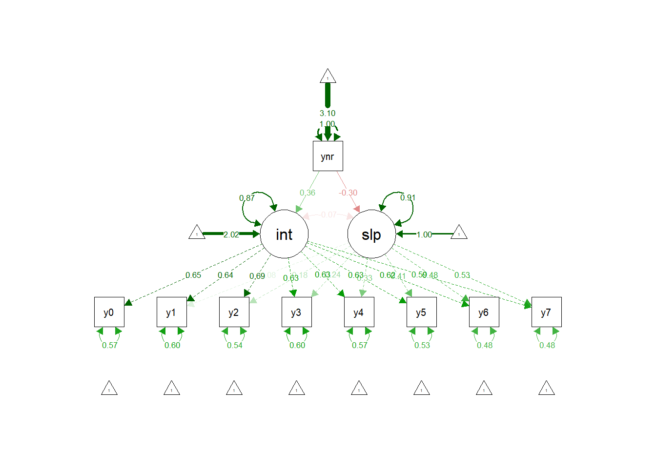
Adding a Continuous Latent Predictor to the LGC Model
By adding the measured neurotic variables to the LGCM of stress (continuous or categorical), we are simply conducting an analysis that is, to all intents and purposes, the same as multilevel modeling. We are also, importantly, using predict variables that contain measurement error. We know this is problematic for estimates.
The major advantage of the LGCM approach is that we can add latent predictors which, as we know, are measured without error. Unfortunately, the Ram et al stress data set does not contain any item level data - just the averaged measures. No problem, we can simply simulate three correlated variables and merge them to our stress_wide dataset. Let’s quickly do that now:
require(MASS)## Loading required package: MASS##
## Attaching package: 'MASS'## The following object is masked from 'package:dplyr':
##
## selectout <- mvrnorm(191, mu = c(0,0,0), Sigma = matrix(c(1,0.65,0.65,0.65,1,0.65,0.65,0.65,1), ncol = 3),
empirical = TRUE)
out <- as.data.frame(out)
stress_wide$v1 <- out$V1
stress_wide$v2 <- out$V2
stress_wide$v3 <- out$V3Great, we now have 3 new random correlated variables, v1, v2, and v3, in the stress_wide dataset. Let’s say for the sake our our example they are the neuroticism items. Remember, they are random, so we should not expect them to be correlated with stress. This example is simply to show you how the analysis is done and the interpretation of the output.
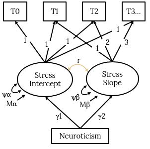
When a latent variable predictor is in the model, the LGCM looks like below, with the predictor represented by a latent variable that is the common variance of its items (i.e., measured without error).
LGCM of Stress with Latent Variable Predictor
Build the LGCM model with Latent Predictor
All we do to add our latent predictor to the LGCM model is create it as a new latent variable using =~ and then regress it on the intercept and slope latent variables using ~. Simple!
lgc.lat.model <- "
    # intercept and slope with fixed coefficients
    intercept =~ 1*y0 + 1*y1 + 1*y2 + 1*y3 + 1*y4 + 1*y5 + 1*y6 + 1*y7
    slope =~ 0*y0 + 1*y1 + 2*y2 + 3*y3 + 4*y4 + 5*y5 + 6*y6 + 7*y7
    # latent neuroticism predictor variable
    neuroticism =~ 1*v1 + v2 + v3
    # regress latent variable predictor on the slopes and intercepts
    intercept ~ neuroticism
    slope ~ neuroticism
"
Now lets fit that model in exactly the same way we did for the categorical and continuous predictors:
lgc.lat.fit <- growth(lgc.lat.model, data=stress_wide, se = "bootstrap", bootstrap = 100)
summary(lgc.lat.fit, fit.measures=TRUE, standardized=TRUE)
## lavaan 0.6-7 ended normally after 43 iterations
##
## Estimator ML
## Optimization method NLMINB
## Number of free parameters 22
##
## Used Total
## Number of observations 159 191
##
## Model Test User Model:
##
## Test statistic 88.804
## Degrees of freedom 55
## P-value (Chi-square) 0.003
##
## Model Test Baseline Model:
##
## Test statistic 684.226
## Degrees of freedom 55
## P-value 0.000
##
## User Model versus Baseline Model:
##
## Comparative Fit Index (CFI) 0.946
## Tucker-Lewis Index (TLI) 0.946
##
## Loglikelihood and Information Criteria:
##
## Loglikelihood user model (H0) -1697.113
## Loglikelihood unrestricted model (H1) -1652.711
##
## Akaike (AIC) 3438.226
## Bayesian (BIC) 3505.742
## Sample-size adjusted Bayesian (BIC) 3436.100
##
## Root Mean Square Error of Approximation:
##
## RMSEA 0.062
## 90 Percent confidence interval - lower 0.037
## 90 Percent confidence interval - upper 0.085
## P-value RMSEA <= 0.05 0.193
##
## Standardized Root Mean Square Residual:
##
## SRMR 0.071
##
## Parameter Estimates:
##
## Standard errors Bootstrap
## Number of requested bootstrap draws 100
## Number of successful bootstrap draws 100
##
## Latent Variables:
## Estimate Std.Err z-value P(>|z|) Std.lv Std.all
## intercept =~
## y0 1.000 0.435 0.646
## y1 1.000 0.435 0.640
## y2 1.000 0.435 0.688
## y3 1.000 0.435 0.633
## y4 1.000 0.435 0.630
## y5 1.000 0.435 0.626
## y6 1.000 0.435 0.621
## y7 1.000 0.435 0.590
## slope =~
## y0 0.000 0.000 0.000
## y1 1.000 0.056 0.082
## y2 2.000 0.111 0.176
## y3 3.000 0.167 0.243
## y4 4.000 0.223 0.323
## y5 5.000 0.279 0.401
## y6 6.000 0.334 0.478
## y7 7.000 0.390 0.529
## neuroticism =~
## v1 1.000 0.794 0.804
## v2 1.011 0.107 9.441 0.000 0.802 0.817
## v3 1.002 0.109 9.216 0.000 0.795 0.794
##
## Regressions:
## Estimate Std.Err z-value P(>|z|) Std.lv Std.all
## intercept ~
## neuroticism -0.004 0.048 -0.083 0.933 -0.007 -0.007
## slope ~
## neuroticism -0.000 0.011 -0.035 0.972 -0.005 -0.005
##
## Covariances:
## Estimate Std.Err z-value P(>|z|) Std.lv Std.all
## .intercept ~~
## .slope -0.004 0.005 -0.762 0.446 -0.161 -0.161
##
## Intercepts:
## Estimate Std.Err z-value P(>|z|) Std.lv Std.all
## .y0 0.000 0.000 0.000
## .y1 0.000 0.000 0.000
## .y2 0.000 0.000 0.000
## .y3 0.000 0.000 0.000
## .y4 0.000 0.000 0.000
## .y5 0.000 0.000 0.000
## .y6 0.000 0.000 0.000
## .y7 0.000 0.000 0.000
## .v1 0.000 0.000 0.000
## .v2 0.000 0.000 0.000
## .v3 0.000 0.000 0.000
## .intercept 1.360 0.042 32.646 0.000 3.130 3.130
## .slope 0.004 0.008 0.485 0.627 0.069 0.069
## neuroticism -0.037 0.072 -0.523 0.601 -0.047 -0.047
##
## Variances:
## Estimate Std.Err z-value P(>|z|) Std.lv Std.all
## .y0 0.264 0.040 6.617 0.000 0.264 0.583
## .y1 0.277 0.051 5.447 0.000 0.277 0.601
## .y2 0.213 0.025 8.686 0.000 0.213 0.535
## .y3 0.278 0.046 5.992 0.000 0.278 0.590
## .y4 0.269 0.038 7.082 0.000 0.269 0.565
## .y5 0.255 0.032 7.870 0.000 0.255 0.529
## .y6 0.236 0.032 7.395 0.000 0.236 0.482
## .y7 0.256 0.042 6.080 0.000 0.256 0.473
## .v1 0.345 0.056 6.109 0.000 0.345 0.354
## .v2 0.320 0.066 4.816 0.000 0.320 0.332
## .v3 0.371 0.073 5.101 0.000 0.371 0.370
## .intercept 0.189 0.032 5.962 0.000 1.000 1.000
## .slope 0.003 0.001 2.717 0.007 1.000 1.000
## neuroticism 0.630 0.118 5.354 0.000 1.000 1.000parameterestimates(lgc.lat.fit, boot.ci.type = "perc", standardized = TRUE)## lhs op rhs est se z pvalue ci.lower ci.upper
## 1 intercept =~ y0 1.000 0.000 NA NA 1.000 1.000
## 2 intercept =~ y1 1.000 0.000 NA NA 1.000 1.000
## 3 intercept =~ y2 1.000 0.000 NA NA 1.000 1.000
## 4 intercept =~ y3 1.000 0.000 NA NA 1.000 1.000
## 5 intercept =~ y4 1.000 0.000 NA NA 1.000 1.000
## 6 intercept =~ y5 1.000 0.000 NA NA 1.000 1.000
## 7 intercept =~ y6 1.000 0.000 NA NA 1.000 1.000
## 8 intercept =~ y7 1.000 0.000 NA NA 1.000 1.000
## 9 slope =~ y0 0.000 0.000 NA NA 0.000 0.000
## 10 slope =~ y1 1.000 0.000 NA NA 1.000 1.000
## 11 slope =~ y2 2.000 0.000 NA NA 2.000 2.000
## 12 slope =~ y3 3.000 0.000 NA NA 3.000 3.000
## 13 slope =~ y4 4.000 0.000 NA NA 4.000 4.000
## 14 slope =~ y5 5.000 0.000 NA NA 5.000 5.000
## 15 slope =~ y6 6.000 0.000 NA NA 6.000 6.000
## 16 slope =~ y7 7.000 0.000 NA NA 7.000 7.000
## 17 neuroticism =~ v1 1.000 0.000 NA NA 1.000 1.000
## 18 neuroticism =~ v2 1.011 0.107 9.441 0.000 0.858 1.292
## 19 neuroticism =~ v3 1.002 0.109 9.216 0.000 0.808 1.271
## 20 intercept ~ neuroticism -0.004 0.048 -0.083 0.933 -0.113 0.108
## 21 slope ~ neuroticism 0.000 0.011 -0.035 0.972 -0.023 0.022
## 22 y0 ~~ y0 0.264 0.040 6.617 0.000 0.202 0.355
## 23 y1 ~~ y1 0.277 0.051 5.447 0.000 0.186 0.394
## 24 y2 ~~ y2 0.213 0.025 8.686 0.000 0.172 0.267
## 25 y3 ~~ y3 0.278 0.046 5.992 0.000 0.188 0.383
## 26 y4 ~~ y4 0.269 0.038 7.082 0.000 0.197 0.352
## 27 y5 ~~ y5 0.255 0.032 7.870 0.000 0.185 0.310
## 28 y6 ~~ y6 0.236 0.032 7.395 0.000 0.173 0.300
## 29 y7 ~~ y7 0.256 0.042 6.080 0.000 0.178 0.347
## 30 v1 ~~ v1 0.345 0.056 6.109 0.000 0.220 0.438
## 31 v2 ~~ v2 0.320 0.066 4.816 0.000 0.193 0.454
## 32 v3 ~~ v3 0.371 0.073 5.101 0.000 0.199 0.519
## 33 intercept ~~ intercept 0.189 0.032 5.962 0.000 0.128 0.254
## 34 slope ~~ slope 0.003 0.001 2.717 0.007 0.000 0.005
## 35 neuroticism ~~ neuroticism 0.630 0.118 5.354 0.000 0.398 0.892
## 36 intercept ~~ slope -0.004 0.005 -0.762 0.446 -0.015 0.007
## 37 y0 ~1 0.000 0.000 NA NA 0.000 0.000
## 38 y1 ~1 0.000 0.000 NA NA 0.000 0.000
## 39 y2 ~1 0.000 0.000 NA NA 0.000 0.000
## 40 y3 ~1 0.000 0.000 NA NA 0.000 0.000
## 41 y4 ~1 0.000 0.000 NA NA 0.000 0.000
## 42 y5 ~1 0.000 0.000 NA NA 0.000 0.000
## 43 y6 ~1 0.000 0.000 NA NA 0.000 0.000
## 44 y7 ~1 0.000 0.000 NA NA 0.000 0.000
## 45 v1 ~1 0.000 0.000 NA NA 0.000 0.000
## 46 v2 ~1 0.000 0.000 NA NA 0.000 0.000
## 47 v3 ~1 0.000 0.000 NA NA 0.000 0.000
## 48 intercept ~1 1.360 0.042 32.646 0.000 1.290 1.451
## 49 slope ~1 0.004 0.008 0.485 0.627 -0.012 0.020
## 50 neuroticism ~1 -0.037 0.072 -0.523 0.601 -0.155 0.131
## std.lv std.all std.nox
## 1 0.435 0.646 0.646
## 2 0.435 0.640 0.640
## 3 0.435 0.688 0.688
## 4 0.435 0.633 0.633
## 5 0.435 0.630 0.630
## 6 0.435 0.626 0.626
## 7 0.435 0.621 0.621
## 8 0.435 0.590 0.590
## 9 0.000 0.000 0.000
## 10 0.056 0.082 0.082
## 11 0.111 0.176 0.176
## 12 0.167 0.243 0.243
## 13 0.223 0.323 0.323
## 14 0.279 0.401 0.401
## 15 0.334 0.478 0.478
## 16 0.390 0.529 0.529
## 17 0.794 0.804 0.804
## 18 0.802 0.817 0.817
## 19 0.795 0.794 0.794
## 20 -0.007 -0.007 -0.007
## 21 -0.005 -0.005 -0.005
## 22 0.264 0.583 0.583
## 23 0.277 0.601 0.601
## 24 0.213 0.535 0.535
## 25 0.278 0.590 0.590
## 26 0.269 0.565 0.565
## 27 0.255 0.529 0.529
## 28 0.236 0.482 0.482
## 29 0.256 0.473 0.473
## 30 0.345 0.354 0.354
## 31 0.320 0.332 0.332
## 32 0.371 0.370 0.370
## 33 1.000 1.000 1.000
## 34 1.000 1.000 1.000
## 35 1.000 1.000 1.000
## 36 -0.161 -0.161 -0.161
## 37 0.000 0.000 0.000
## 38 0.000 0.000 0.000
## 39 0.000 0.000 0.000
## 40 0.000 0.000 0.000
## 41 0.000 0.000 0.000
## 42 0.000 0.000 0.000
## 43 0.000 0.000 0.000
## 44 0.000 0.000 0.000
## 45 0.000 0.000 0.000
## 46 0.000 0.000 0.000
## 47 0.000 0.000 0.000
## 48 3.130 3.130 3.130
## 49 0.069 0.069 0.069
## 50 -0.047 -0.047 -0.047First of all, again, the model fit looks pretty good. We have CFI = .97, TLI .97, RMSEA = .05, and SRMR = .06. The standardised factor loadings for the neuroticism latent variable are also all above .40, which means the measurement is good. Of interest here are the regressions, first of the latent stress intercept on latent neuroticism variable and second of the latent stress slope on latent neuroticism variable.
We can see that the regression of stress intercepts on neuroticism is .02 and this is a non-significant effect according the the 95% bootstrap confidence interval (95% Ci = -.08, .18). We should not be surprised by this, the items were simulated randomly and therefor these is no reason to expect any relationship. The interpretation of this regression is that for every one unit increase in the latent neuroticism variable there is a .02 unit increase in the stress starting point (i.e., time point 0). Interesting, again, but what we really want to know is whether the trajectories of stress differ across the range of neuroticism.
To answer that question we need to look to the regression of stress slopes on the latent neuroticism variable. Here we have an estimate of -.01 and this is not a significant effect according the the 95% bootstrap confidence interval (95% Ci = -.03, .01). As with the intercept regression, we should expect this given the random simulation of the neuroticism items. The interpretation of this regression is that for every one unit increase in neuroticism the trajectory slopes of stress decrease by .01. This is not a significant decrease.
We can visualize this model using SEM plot:
semPaths(lgc.lat.fit, "std")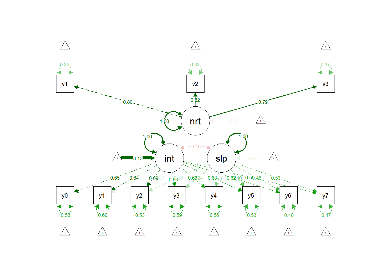
The difference here being neuroticism is reflected by a latent variable, rather than a measured one.
Okay, that is it. That is how we do LGCM with categorical, continuous and latent variable predictors.
Activity: Reading Ability Dataset
In the example we will work with for this activity, we use an dataset called Demo.growth from the lavaan package, where a standardized score on a reading ability scale is measured on 4 time points among kindergarten children in the US (t1, t2, t3, t4. There are also a couple of predictors in this dataset that we might use to predict the intercepts and slopes in reading ability:
x1 Parent Support
x2 Teacher Support
We will build a model that uses the measure of parent support to predict the intercepts and slopes of reading ability.
We expect that parent support would exhibit a positive relationship with the intercepts and slopes of reading ability.
Load data
Luckily, the Political Democracy dataset is a practice dataset contained in the lavaan package for CFA, so we don’t need to load it from the computer, we can load it from the package. Lets do that now and save it as object called “pol”:
reading <- lavaan::Demo.growth
head(reading)
## t1 t2 t3 t4 x1 x2
## 1 1.7256454 2.1424005 2.7731717 2.51595586 -1.1641026 0.1742293
## 2 -1.9841595 -4.4006027 -6.0165563 -7.02961801 -1.7454025 -1.5768602
## 3 0.3195183 -1.2691171 1.5600160 2.86852958 0.9202112 -0.1418180
## 4 0.7769485 3.5313707 3.1382114 5.36374139 2.3595236 0.7079681
## 5 0.4489440 -0.7727747 -1.5035150 0.07846742 -1.0887077 -1.0099977
## 6 -1.7469951 -0.9963400 -0.8242174 0.56692480 -0.5135169 -0.1440428
## c1 c2 c3 c4
## 1 -0.02767765 0.5549234 0.2544784 -1.00639541
## 2 -2.03196724 0.1253348 -1.5642323 1.22926875
## 3 0.05237496 -1.2577408 -1.8033909 -0.32725761
## 4 0.01911429 0.6473830 -0.4323795 -1.03239779
## 5 0.65243274 0.7309148 -0.7537816 -0.02745598
## 6 -0.04452906 -0.4168022 -1.2411670 0.51719763Building and Fitting the LGC Model of Reading Ability
Before we test the relationships between support and reading ability, we first need to take a look at the growth model of reading ability, to make sure that there is intercept and slope variance to be explained.
To do that we need to first build the simple growth model of reading ability that contains no predictors. Write the code to build the LGM of reading ability and save it as a new object called lgc.reading (don’t forget to fix the factors loadings appropriately):
lgc.reading <- "
    intercept =~ 1*t1 + 1*t2 + 1*t3 + 1*t4
    slope =~ 0*t1 + 1*t2 + 2*t3 + 3*t4
"
Now fit that LGCM of reading ability to the data. Don’t forget to use the growth() function and save the new object as reading.fit:
reading.fit <- growth(lgc.reading, data=reading)
summary(reading.fit, fit.measures=TRUE, standardized=TRUE)
## lavaan 0.6-7 ended normally after 29 iterations
##
## Estimator ML
## Optimization method NLMINB
## Number of free parameters 9
##
## Number of observations 400
##
## Model Test User Model:
##
## Test statistic 8.069
## Degrees of freedom 5
## P-value (Chi-square) 0.152
##
## Model Test Baseline Model:
##
## Test statistic 1780.035
## Degrees of freedom 6
## P-value 0.000
##
## User Model versus Baseline Model:
##
## Comparative Fit Index (CFI) 0.998
## Tucker-Lewis Index (TLI) 0.998
##
## Loglikelihood and Information Criteria:
##
## Loglikelihood user model (H0) -2755.052
## Loglikelihood unrestricted model (H1) -2751.018
##
## Akaike (AIC) 5528.104
## Bayesian (BIC) 5564.027
## Sample-size adjusted Bayesian (BIC) 5535.470
##
## Root Mean Square Error of Approximation:
##
## RMSEA 0.039
## 90 Percent confidence interval - lower 0.000
## 90 Percent confidence interval - upper 0.087
## P-value RMSEA <= 0.05 0.580
##
## Standardized Root Mean Square Residual:
##
## SRMR 0.012
##
## Parameter Estimates:
##
## Standard errors Standard
## Information Expected
## Information saturated (h1) model Structured
##
## Latent Variables:
## Estimate Std.Err z-value P(>|z|) Std.lv Std.all
## intercept =~
## t1 1.000 1.390 0.874
## t2 1.000 1.390 0.660
## t3 1.000 1.390 0.511
## t4 1.000 1.390 0.411
## slope =~
## t1 0.000 0.000 0.000
## t2 1.000 0.766 0.364
## t3 2.000 1.532 0.564
## t4 3.000 2.298 0.680
##
## Covariances:
## Estimate Std.Err z-value P(>|z|) Std.lv Std.all
## intercept ~~
## slope 0.618 0.071 8.686 0.000 0.580 0.580
##
## Intercepts:
## Estimate Std.Err z-value P(>|z|) Std.lv Std.all
## .t1 0.000 0.000 0.000
## .t2 0.000 0.000 0.000
## .t3 0.000 0.000 0.000
## .t4 0.000 0.000 0.000
## intercept 0.615 0.077 8.007 0.000 0.442 0.442
## slope 1.006 0.042 24.076 0.000 1.314 1.314
##
## Variances:
## Estimate Std.Err z-value P(>|z|) Std.lv Std.all
## .t1 0.595 0.086 6.944 0.000 0.595 0.236
## .t2 0.676 0.061 11.061 0.000 0.676 0.153
## .t3 0.635 0.072 8.761 0.000 0.635 0.086
## .t4 0.508 0.124 4.090 0.000 0.508 0.044
## intercept 1.932 0.173 11.194 0.000 1.000 1.000
## slope 0.587 0.052 11.336 0.000 1.000 1.000Summarize the model fit for this LGCM, does it fit the data well?
What is the fixed effect for the intercept? What does this mean?
What is the fixed effect for the slope? What does this mean?
What is the random effect for the intercept? Is it significant? What does this mean?
What is the random effect for the slope? Is it significant? What does this mean?
What is the covariance between the intercepts and slopes? What does this mean?
Adding a Predictor Variable
Okay so we have significant variability around our fixed intercepts and slopes of reading ability. As we know, this means that there is substantial between-child variability in starting points of reading ability (intercepts) as well as in the positive change trajectories of reading ability (slopes). To see if support can explain any variability in these intercepts and slopes, lets regress the random intercepts and slopes of reading ability on parent support (x1).
First, write the code that builds this LGCM with the parent support predictor. Recall that parent support in the dataset is the x1 variable. Call the model object lgc.reading.model:
lgc.reading.model <- "
    intercept =~ 1*t1 + 1*t2 + 1*t3 + 1*t4
    slope =~ 0*t1 + 1*t2 + 2*t3 + 3*t4
    intercept ~ x1
    slope ~ x1
"
No write the code to fit that model to the data and save the new object as lgc.reading.fit. Don’t forget to bootstrap the standard errors and request the parameter estimates:
## Fit the lgc.reading.model
lgc.reading.fit <- growth(lgc.reading.model, data=reading, se = "bootstrap", bootstrap = 100)

## Summarize the fitted model
summary(lgc.reading.fit, fit.measures=TRUE, standardized=TRUE)
## lavaan 0.6-7 ended normally after 28 iterations
##
## Estimator ML
## Optimization method NLMINB
## Number of free parameters 11
##
## Number of observations 400
##
## Model Test User Model:
##
## Test statistic 8.207
## Degrees of freedom 7
## P-value (Chi-square) 0.315
##
## Model Test Baseline Model:
##
## Test statistic 1918.127
## Degrees of freedom 10
## P-value 0.000
##
## User Model versus Baseline Model:
##
## Comparative Fit Index (CFI) 0.999
## Tucker-Lewis Index (TLI) 0.999
##
## Loglikelihood and Information Criteria:
##
## Loglikelihood user model (H0) -2686.075
## Loglikelihood unrestricted model (H1) -2681.971
##
## Akaike (AIC) 5394.150
## Bayesian (BIC) 5438.056
## Sample-size adjusted Bayesian (BIC) 5403.152
##
## Root Mean Square Error of Approximation:
##
## RMSEA 0.021
## 90 Percent confidence interval - lower 0.000
## 90 Percent confidence interval - upper 0.067
## P-value RMSEA <= 0.05 0.812
##
## Standardized Root Mean Square Residual:
##
## SRMR 0.010
##
## Parameter Estimates:
##
## Standard errors Bootstrap
## Number of requested bootstrap draws 100
## Number of successful bootstrap draws 100
##
## Latent Variables:
## Estimate Std.Err z-value P(>|z|) Std.lv Std.all
## intercept =~
## t1 1.000 1.390 0.875
## t2 1.000 1.390 0.661
## t3 1.000 1.390 0.511
## t4 1.000 1.390 0.411
## slope =~
## t1 0.000 0.000 0.000
## t2 1.000 0.767 0.364
## t3 2.000 1.533 0.564
## t4 3.000 2.300 0.680
##
## Regressions:
## Estimate Std.Err z-value P(>|z|) Std.lv Std.all
## intercept ~
## x1 0.698 0.069 10.071 0.000 0.502 0.516
## slope ~
## x1 0.338 0.038 8.824 0.000 0.441 0.453
##
## Covariances:
## Estimate Std.Err z-value P(>|z|) Std.lv Std.all
## .intercept ~~
## .slope 0.368 0.052 7.105 0.000 0.452 0.452
##
## Intercepts:
## Estimate Std.Err z-value P(>|z|) Std.lv Std.all
## .t1 0.000 0.000 0.000
## .t2 0.000 0.000 0.000
## .t3 0.000 0.000 0.000
## .t4 0.000 0.000 0.000
## .intercept 0.679 0.066 10.294 0.000 0.488 0.488
## .slope 1.037 0.040 26.235 0.000 1.353 1.353
##
## Variances:
## Estimate Std.Err z-value P(>|z|) Std.lv Std.all
## .t1 0.593 0.087 6.820 0.000 0.593 0.235
## .t2 0.676 0.068 9.921 0.000 0.676 0.153
## .t3 0.639 0.066 9.622 0.000 0.639 0.086
## .t4 0.500 0.124 4.021 0.000 0.500 0.044
## .intercept 1.419 0.126 11.251 0.000 0.734 0.734
## .slope 0.467 0.051 9.238 0.000 0.795 0.795## Request the parameter estimates for the 95% bootstrap confidence intervals
parameterestimates(lgc.reading.fit, boot.ci.type = "perc", standardized = TRUE)## lhs op rhs est se z pvalue ci.lower ci.upper std.lv
## 1 intercept =~ t1 1.000 0.000 NA NA 1.000 1.000 1.390
## 2 intercept =~ t2 1.000 0.000 NA NA 1.000 1.000 1.390
## 3 intercept =~ t3 1.000 0.000 NA NA 1.000 1.000 1.390
## 4 intercept =~ t4 1.000 0.000 NA NA 1.000 1.000 1.390
## 5 slope =~ t1 0.000 0.000 NA NA 0.000 0.000 0.000
## 6 slope =~ t2 1.000 0.000 NA NA 1.000 1.000 0.767
## 7 slope =~ t3 2.000 0.000 NA NA 2.000 2.000 1.533
## 8 slope =~ t4 3.000 0.000 NA NA 3.000 3.000 2.300
## 9 intercept ~ x1 0.698 0.069 10.071 0 0.580 0.838 0.502
## 10 slope ~ x1 0.338 0.038 8.824 0 0.252 0.424 0.441
## 11 t1 ~~ t1 0.593 0.087 6.820 0 0.425 0.787 0.593
## 12 t2 ~~ t2 0.676 0.068 9.921 0 0.536 0.847 0.676
## 13 t3 ~~ t3 0.639 0.066 9.622 0 0.477 0.785 0.639
## 14 t4 ~~ t4 0.500 0.124 4.021 0 0.255 0.704 0.500
## 15 intercept ~~ intercept 1.419 0.126 11.251 0 1.159 1.656 0.734
## 16 slope ~~ slope 0.467 0.051 9.238 0 0.375 0.593 0.795
## 17 intercept ~~ slope 0.368 0.052 7.105 0 0.272 0.459 0.452
## 18 x1 ~~ x1 1.056 0.000 NA NA 1.056 1.056 1.056
## 19 t1 ~1 0.000 0.000 NA NA 0.000 0.000 0.000
## 20 t2 ~1 0.000 0.000 NA NA 0.000 0.000 0.000
## 21 t3 ~1 0.000 0.000 NA NA 0.000 0.000 0.000
## 22 t4 ~1 0.000 0.000 NA NA 0.000 0.000 0.000
## 23 x1 ~1 -0.092 0.000 NA NA -0.092 -0.092 -0.092
## 24 intercept ~1 0.679 0.066 10.294 0 0.545 0.827 0.488
## 25 slope ~1 1.037 0.040 26.235 0 0.937 1.108 1.353
## std.all std.nox
## 1 0.875 0.875
## 2 0.661 0.661
## 3 0.511 0.511
## 4 0.411 0.411
## 5 0.000 0.000
## 6 0.364 0.364
## 7 0.564 0.564
## 8 0.680 0.680
## 9 0.516 0.502
## 10 0.453 0.441
## 11 0.235 0.235
## 12 0.153 0.153
## 13 0.086 0.086
## 14 0.044 0.044
## 15 0.734 0.734
## 16 0.795 0.795
## 17 0.452 0.452
## 18 1.000 1.056
## 19 0.000 0.000
## 20 0.000 0.000
## 21 0.000 0.000
## 22 0.000 0.000
## 23 -0.090 -0.092
## 24 0.488 0.488
## 25 1.353 1.353Summarize the model fit for this LGCM, does it fit the data well?
What is the regression estimate for reading ability intercepts on parent support? Is it statistically significant? What does it mean?
What is the regression estimate for reading ability slopes on parent support? Is it statistically significant? What does it mean?
What can we conclude with regard to our original hypothesis? Do children with high parent support experience greater improvement in reading ability over time?
Visualise the LGCM
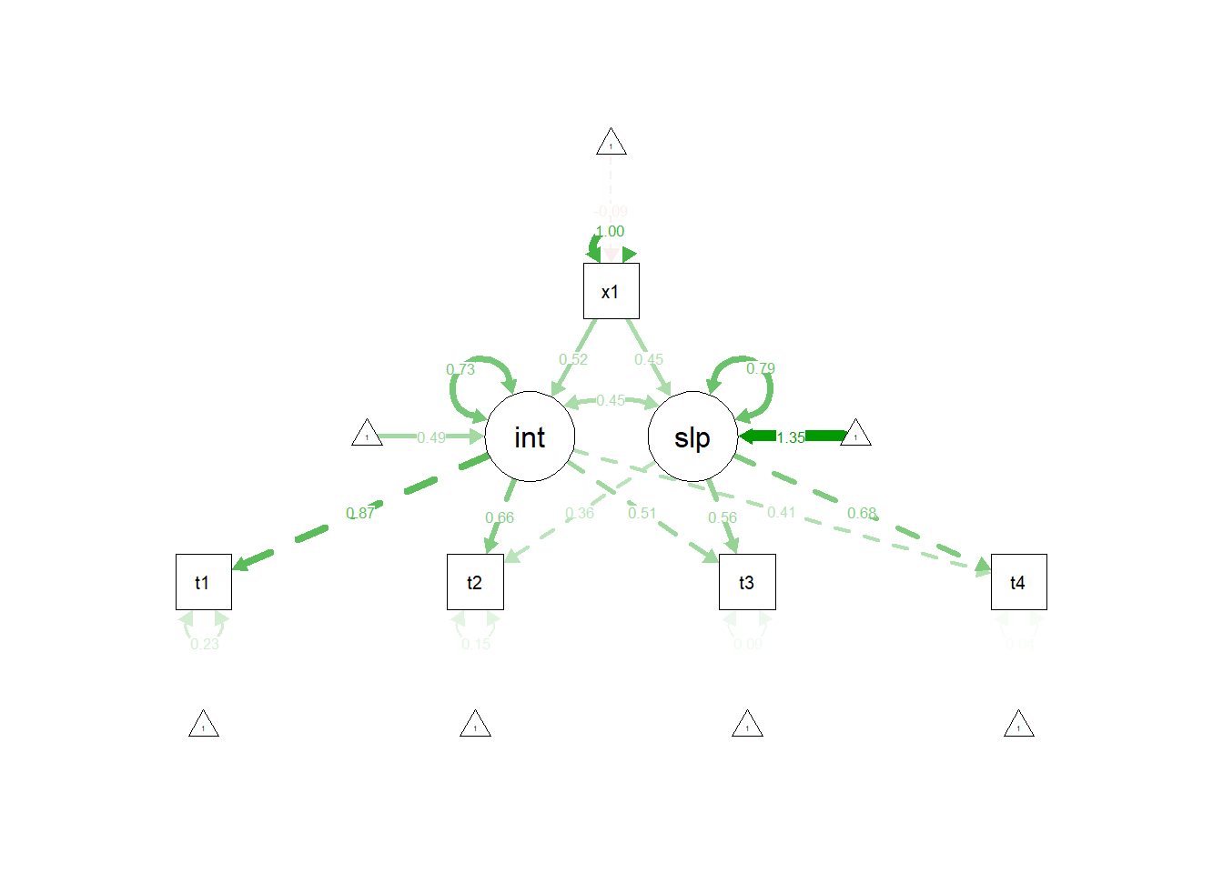
Finally, use semPaths to visualize the LGCM you have just tested:
semPaths(lgc.reading.fit, "std")